
EEG
Explore EEG signals one step at a time. Try three ready-to-open patches and discover what each node can do.
Start exploring without a headset. Explore practice signals in the first recipes, then analyze a real recording with EegPlayback in recipe 3.
Start here
Use goofi 3.1.0 with the EEG and signal bundles available. Open a patch to see its graph, viewers, and controls together in the Explore tab.
The first two recipes use practice EEG signals. Recipe 3 uses EegPlayback to stream a prerecorded eyes-closed EEG sample at its original rate. The sample downloads automatically on first use.
Start with recipe 01 ↓ Bundle setup →
Meet the nodes
Meet the building blocks. See what connects to each node, try a small experiment, or open its documentation for all the settings.
Play an EEG recording
Try it. Choose a recording with playback/file and watch its channels play back. The default scale shows values in microvolts. Use this node when you are ready to replace the practice signals with your own data.
Good to know
The default sample can download on first use. A blank view during that download is expected. Recordings are not included in these recipes.
Inputs: None
Outputs: out: ARRAY
Clean up the signal before you explore
Try it. Change eeg/high from 40 to 30 Hz and look for less fast activity in the trace. The mains setting reduces electrical hum; choose the frequency present in your recording, or 0 to turn it off.
Good to know
Needs channels × fresh samples with sfreq metadata. It withholds the first two seconds after startup or a filter change. Put it before a rolling buffer.
Inputs: input: ARRAY
Outputs: out: ARRAY
Compare different reference signals
Try it. Try none, average, and median under reference/mode. Watch how subtracting a shared reference changes the traces and the relationships between channels.
Good to know
Bipolar mode changes channel count. Laplacian mode needs matching electrode positions. Exclude omits a channel from the reference calculation; it does not remove that output channel.
Inputs: data: ARRAY · montage: ARRAY
Outputs: data: ARRAY
See how much power each band contains
Try it. Turn bands/relative on to show each band’s share of the total power. Then narrow the alpha band from 8–13 to 9–11 Hz and see how much of the 10 Hz peak it still captures.
Good to know
Takes a linear PSD with frequency labels, not a raw waveform or log spectrum. The denominator is the whole supplied spectrum; cropping it changes relative power.
Inputs: psd: ARRAY
Outputs: power: ARRAY
Find peaks above the spectral background
Try it. Look at peaks for the rhythms found in the spectrum, and aperiodic for the fitted background. Try fixed and knee modes to compare two ways of fitting that background.
Good to know
Needs linear spectral power. Missing peaks are NaN-padded; a failed fit also returns NaN. A fitted component alone does not identify a physiological state.
Inputs: psd: ARRAY
Outputs: aperiodic: ARRAY · peaks: ARRAY
Discover which channels change together
Try it. Start with Pearson to compare the shapes of the signals. Then try PLV and wPLI, which compare their timing within a frequency band. Keep the band at 8–13 Hz while you explore.
Good to know
Methods measure different relationships. A shared synthetic oscillator can create high coupling without interaction. Phase methods need a meaningful band and sample rate.
Inputs: data: ARRAY
Outputs: matrix: ARRAY
Explore the network between channels
Try it. Move graph/density from 0.25 to 0.75 to keep more connections. Watch degree to see how connected each channel is, and efficiency to see how easily the network can be traversed.
Good to know
Density 0 disables thresholding. Tied weights can keep extra edges. Path length uses the largest connected component; efficiency includes the full graph.
Inputs: matrix: ARRAY
Outputs: clustering: ARRAY · path: ARRAY · efficiency: ARRAY · betweenness: ARRAY · degree: ARRAY · assortativity: ARRAY · transitivity: ARRAY
Make a clearer picture by averaging
Try it. Compare latest, the newest window, with erp, the running average. Watch count grow as more windows arrive. Press epoch/reset to start again, and try whole under baseline to center each trace around zero.
Good to know
Each qualifying trigger captures the supplied window once. This node does not locate an event within a stream or construct pre/post-event windows. Rejection uses input amplitude units.
Inputs: data: ARRAY · trigger: ARRAY
Outputs: erp: ARRAY · latest: ARRAY · count: ARRAY
Three patch recipes
A spectrum, then its bands
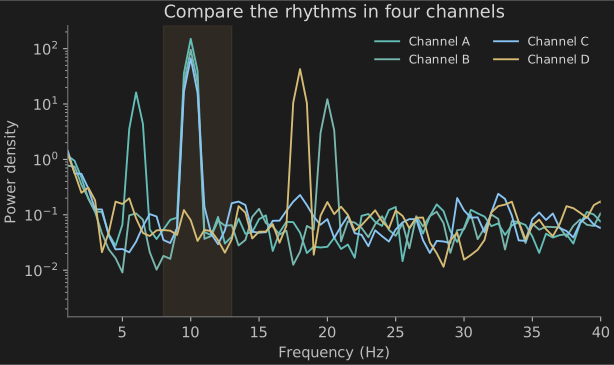
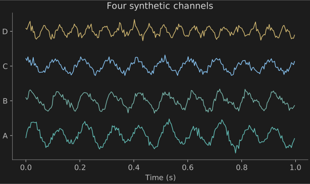
Start with four practice signals that contain a strong 10 Hz rhythm. Follow them through a filter and a reference, then see where their power appears in the spectrum and frequency bands.
Download patch ↓CookbookEeg → EegPreprocess → Reference → Psd → EegPowerBands + Fooof
| Control | Experiment |
|---|---|
| source · signal/alpha | Move 15 → 5 → 25. Compare the 10 Hz peak and relative alpha power. |
| reference · reference/mode | Compare average with none. The reference changes the signal that every downstream analysis sees. |
| bands · bands/relative | Switch between absolute power and a fraction of the 1–40 Hz input spectrum. |
From channels to a network
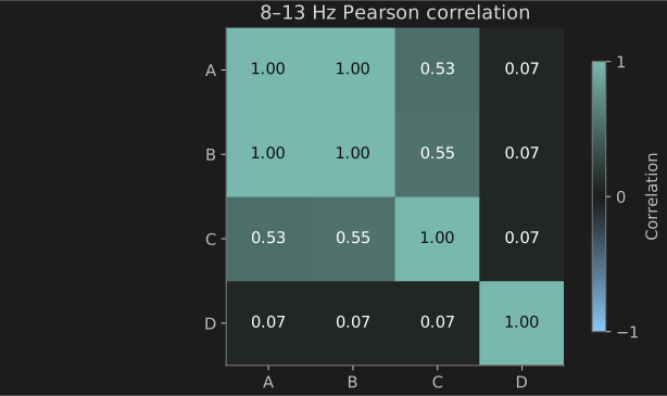
Channels A and B share an oscillator. C has a phase-shifted 10 Hz component; D has an 18 Hz component. Compare the matrix with the network obtained by keeping its strongest relationships.
Download patch ↓CookbookEeg → Reference → Connectivity → GraphMetrics
| Control | Experiment |
|---|---|
| connectivity · connectivity/method | Compare pearson, plv, and wpli. Their values have different meanings. |
| reference · reference/mode | Start at none, then try average. Compare the matrix before changing another control. |
| network · graph/density | Try 0.25, 0.5, and 0.75. Watch the degree display as edges enter the graph. |
Separate peaks from the background
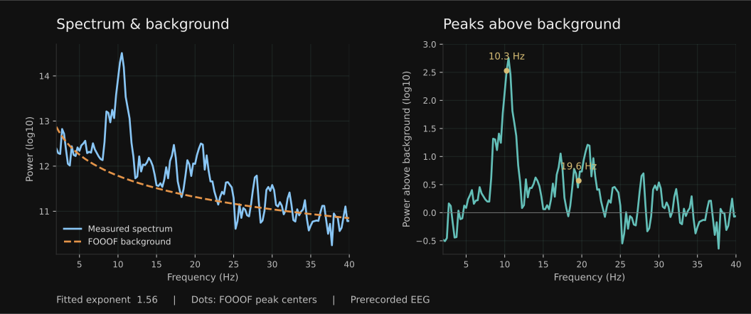
Replay an eyes-closed EEG recording and inspect one channel at a time. Compare its spectrum with the fitted background, then see which peaks rise above it. The two plots update together while the recording plays.
Download patch ↓EegPlayback → Select → Buffer → Psd → Fooof → FooofView
| Control | Experiment |
|---|---|
| Channel | Start with O1, then try Oz or O2. After switching, allow eight seconds for the rolling window to refill. |
| MaximumPeaks | Start with two peaks, then allow more. Compare the detected centers with the visible bumps in the spectrum. |
| MinimumWidth | Increase the minimum width to avoid fitting very narrow fluctuations. Compare the result across several windows. |
Nodes: EegPlaybackFooof
Working practice
Move to a recording
Replace CookbookEeg with EegPlayback. Choose your file, retain its actual sample rate, and select EEG channels before analysis if the recording includes other sensors. For recipe 01, use EegPlayback → EegPreprocess → Reference → Buffer → Psd. Choose samples for Buffer’s unit and set its size to four times the recording’s sample rate. Keep preprocessing before the rolling buffer so each new sample is filtered once.
For connectivity, buffer a complete multichannel window before Connectivity. For Epoch, supply an explicit capture trigger and a complete window; the playback node does not provide event markers. Compare windows from the same condition, reference, channel set, and units.
Read the result in context
Check the raw traces before interpreting a spectrum or matrix. Changes in reference, filtering, window length, or amplitude units change the result. Band power and coupling values alone do not establish a mental state or a diagnosis.
Source revision and file hashes · Synthetic source · All cookbooks