
Simulation
Explore how simple rules create motion, synchronization, memory, and patterns.
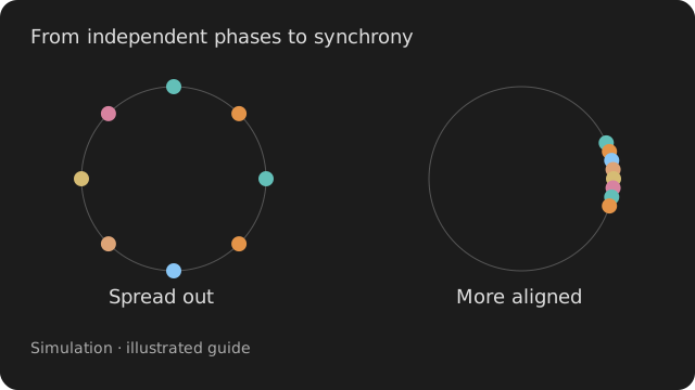
Start a model, watch its output, and change one rule. The signal nodes calculate the simulation. Their matching graphics nodes turn its state into a picture.
Start here
Enable Simulation and Signal. Enable the graphics engine to use the matching display nodes. The numeric outputs can also be explored with line and image viewers.
Open a recipe to see the patch, viewers, and controls together in the Explore tab. The model produces numeric data; its matching graphics node displays that data.
Open the first recipe ↓ Bundle setup →
Meet the nodes
Use the node pictures to find the inputs and outputs. Each experiment points to a recipe you can build on.
Explore a changing trajectory
Try it. Compare lorenz and rossler under attractor/system. Keep a, b, and c at 1 to start.
Good to know
Some systems can settle or become periodic at particular settings. A changing trace alone does not prove chaos.
Inputs: None
Outputs: out: ARRAY
Explore a nonlinear cycle
Try it. Compare vanderpol and duffing under oscillator/model, then change oscillator/nonlinearity.
Good to know
Models interpret the shared controls differently. Reset after changing models before comparing traces.
Inputs: drive: ARRAY
Outputs: out: ARRAY
Follow interacting populations
Try it. Start with lotkavolterra and watch how its two components rise and fall.
Good to know
These are simplified models. Their variables are not forecasts of a real ecosystem or epidemic.
Inputs: None
Outputs: out: ARRAY
Let oscillators fall into step
Try it. Raise kuramoto/coupling from 0 to 3 and watch order.
Good to know
Order near 1 means phases are aligned. Noise and the spread of natural frequencies affect whether alignment occurs.
Inputs: frequencies: ARRAY · coupling: ARRAY
Outputs: phases: ARRAY · waveforms: ARRAY · order: ARRAY
Explore a network of on/off rules
Try it. Compare boolean/connections at 1, 2, and 3, resetting between runs.
Good to know
Activity measures changing units. A fixed seed helps compare the generated networks.
Inputs: None
Outputs: state: ARRAY · activity: ARRAY
Watch activity spread in cascades
Try it. Compare branching/branching below and above 1 while watching activity.
Good to know
Avalanche sizes are reported when a cascade finishes. A short run is not enough to infer a power law or criticality.
Inputs: drive: ARRAY
Outputs: state: ARRAY · activity: ARRAY · avalanche: ARRAY
Explore an associative memory
Try it. Start with its internally generated patterns and compare hopfield/mode values classic and modern.
Good to know
Wire patterns and cue for a controlled recall experiment. The default demonstration does not measure memory accuracy on your own data.
Inputs: patterns: ARRAY · cue: ARRAY
Outputs: state: ARRAY · overlap: ARRAY · energy: ARRAY
Grow trails from local movement
Try it. Change physarum/decay and watch how long trails remain visible.
Good to know
The trail field and agent positions are separate outputs. More agents and a larger field increase processing cost.
Inputs: attract: ARRAY
Outputs: trail: ARRAY · positions: ARRAY
Explore collective movement
Try it. Compare boids and vicsek under swarm/model, then change alignment.
Good to know
The controls apply differently across models. Reset between comparisons and begin with a modest count.
Inputs: attraction: ARRAY
Outputs: positions: ARRAY · velocities: ARRAY · phases: ARRAY · order: ARRAY
Turn an input into a changing internal state
Try it. Change reservoir/leak and watch how quickly state responds.
Good to know
The reservoir is not trained here. Readout learns a mapping from its state to a target.
Inputs: input: ARRAY · connectivity: ARRAY
Outputs: state: ARRAY
Learn a target from a state
Try it. Watch error, then turn readout/learning off to hold the learned weights.
Good to know
This recipe reconstructs its current input. Low training error does not show that it can predict unseen data or the future.
Inputs: state: ARRAY · target: ARRAY
Outputs: prediction: ARRAY · error: ARRAY · weights: ARRAY
Model a population as a few variables
Try it. Compare mass/model values jansenrit and wilsoncowan, then change mass/drive.
Good to know
These are model variables. To analyse their spectrum, retain the sample rate and collect a complete window.
Inputs: input: ARRAY · connectivity: ARRAY
Outputs: out: ARRAY
Explore individual spikes
Try it. Increase neuron/drive gradually and watch rate beside potentials.
Good to know
Network size and time step affect cost and behaviour. Keep them fixed when comparing drive or coupling.
Inputs: input: ARRAY
Outputs: potentials: ARRAY · spikes: ARRAY · rate: ARRAY
Explore a small simulated quantum state
Try it. Change quantum/angle, then compare quantum/entangle on and off.
Good to know
This runs a classical simulation of a quantum state. The state size grows quickly with qubit count.
Inputs: angles: ARRAY
Outputs: probabilities: ARRAY · bloch: ARRAY · entropy: ARRAY
Draw the model’s trajectory
Try it. Connect signal Attractor.out to the graphics node’s out input.
Good to know
The input is named out because it matches the model output. Use a buffered history if you want a longer path.
Inputs: out: ARRAY
Outputs: out: TEXTURE
See phases around a circle
Try it. Connect phases and compare the cluster of dots with the signal node’s order value.
Good to know
The graphics node shows the latest sample of a block. Large populations may be sampled for display.
Inputs: phases: ARRAY
Outputs: out: TEXTURE
See a Boolean network
Try it. Connect state and compare the picture as the model changes its rules.
Good to know
This is a view of the signal model; it does not generate a second network.
Inputs: state: ARRAY
Outputs: out: TEXTURE
See cascades of activity
Try it. Connect state, activity, and avalanche to the matching inputs.
Good to know
Keep all three inputs from the same Branching node so the display describes one run.
Inputs: state: ARRAY · activity: ARRAY · avalanche: ARRAY
Outputs: out: TEXTURE
See memory states
Try it. Connect state and overlap, then compare recall under different settings.
Good to know
The display shows the state supplied by the signal model.
Inputs: state: ARRAY · overlap: ARRAY
Outputs: out: TEXTURE
Render trails and agents
Try it. Connect trail and positions, then compare dense and fading trails.
Good to know
The model creates the field; this node renders it as a texture.
Inputs: trail: ARRAY · positions: ARRAY
Outputs: out: TEXTURE
Render collective movement
Try it. Connect positions, velocities, and phases from one Swarm model.
Good to know
Keep the model in two dimensions for the simplest first view.
Inputs: positions: ARRAY · velocities: ARRAY · phases: ARRAY
Outputs: out: TEXTURE
See the reservoir’s activity
Try it. Connect state and vary the input signal.
Good to know
The picture is a view of internal activations, not a measure of prediction quality.
Inputs: state: ARRAY
Outputs: out: TEXTURE
See spikes and membrane potentials
Try it. Connect spikes and potentials from the same model.
Good to know
Use the signal outputs when you need numeric analysis rather than a rendered picture.
Inputs: spikes: ARRAY · potentials: ARRAY
Outputs: out: TEXTURE
See probabilities and Bloch vectors
Try it. Connect probabilities and bloch while changing the model’s rotation angle.
Good to know
The view describes a simulated state; it does not perform measurements on hardware.
Inputs: bloch: ARRAY · probabilities: ARRAY
Outputs: out: TEXTURE
Patch recipes
Three kinds of changing motion
Compare an attractor, a nonlinear oscillator, and a population model. Each runs independently.
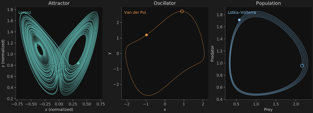
- Open the line viewers on Attractor, Oscillator, and Population. These downloads use block output so each viewer receives several samples.
- Start with the default models and watch how their shapes differ.
- Change one model at a time, then press sim/reset to start it again.
Attractor.outAttractorGraphics.outWhat to look for. The models can oscillate, settle, or change irregularly. Their variables and scales have different meanings.
Switch Attractor from lorenz to rossler. Compare the components, then restore lorenz and change attractor/a slightly.
To draw a longer trajectory, add a Buffer before graphics Attractor and keep the coordinate axis intact.
Oscillators that synchronize
Give oscillators different natural frequencies, then increase their influence on one another.
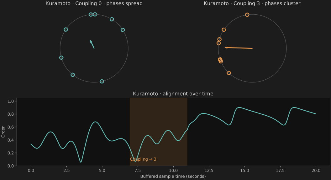
- Start with kuramoto/coupling at 0 and watch the phases spread around the circle.
- Raise coupling to 1, then 3. Give the model time to settle at each setting.
- Compare the circle with the numeric order output.
Kuramoto.phasesKuramotoGraphics.phasesWhat to look for. Stronger coupling can pull phases together. Order approaches 1 as the oscillators align.
Keep coupling fixed and increase kuramoto/spread. Compare the result, then reset with the same seed.
Kuramoto is the signal model; KuramotoGraphics is the matching display node. Open the graphics out texture in a viewer.
Rules, cascades, and memory
Compare three networks with different rules for changing their state.
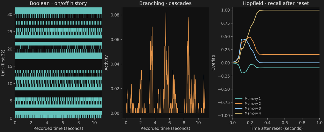
- Watch Boolean.activity for units that keep changing.
- Watch Branching.activity as cascades spread and end.
- Inspect Hopfield.state and overlap to see which internally generated pattern the model approaches.
Boolean.stateBooleanGraphics.stateBranching.stateBranchingGraphics.stateBranching.activityBranchingGraphics.activityBranching.avalancheBranchingGraphics.avalancheHopfield.stateHopfieldGraphics.stateHopfield.overlapHopfieldGraphics.overlapWhat to look for. Similar-looking arrays can describe different systems: on/off rules, spreading events, or an associative memory.
Change one model at a time. Try Boolean connections 1 versus 3, or Branching ratio 0.8 versus 1.2. Reset between runs.
The three graphics nodes display their matching models. Avalanche statistics require many completed events; this recipe introduces the controls.
Trails and flocks
Explore two forms of collective movement: agents that follow trails and particles that follow neighbours.
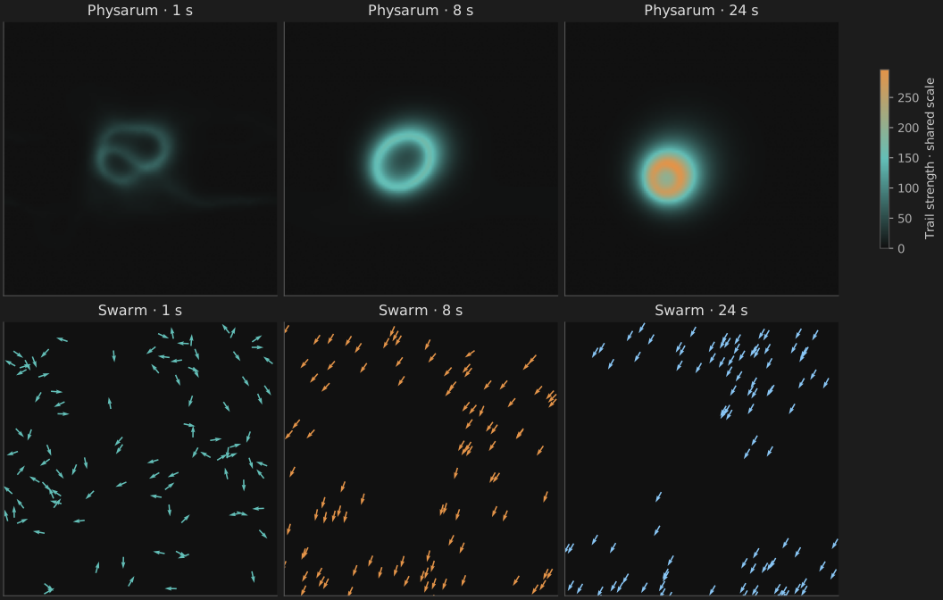
- Open Physarum.trail in an image viewer. Let the trail develop before changing a control.
- Open the graphics outputs to see the rendered models.
- Change physarum/decay or swarm/alignment while keeping the other model fixed.
Physarum.trailPhysarumGraphics.trailPhysarum.positionsPhysarumGraphics.positionsSwarm.positionsSwarmGraphics.positionsSwarm.velocitiesSwarmGraphics.velocitiesSwarm.phasesSwarmGraphics.phasesWhat to look for. Physarum retains a spatial history through its trail field. Swarm updates particles from their interactions.
Raise physarum/decay from 0.005 to 0.08 to shorten the trail memory. In Swarm, compare vicsek with boids and reset before each run.
The starting counts are modest. Physarum starts with long-lived trails and gentle turns; Swarm starts in Vicsek mode so neighbours can align. Increase the counts after the patch runs smoothly.
Learn a simple readout
Drive a reservoir with a slow wave and train a readout to reconstruct that wave.
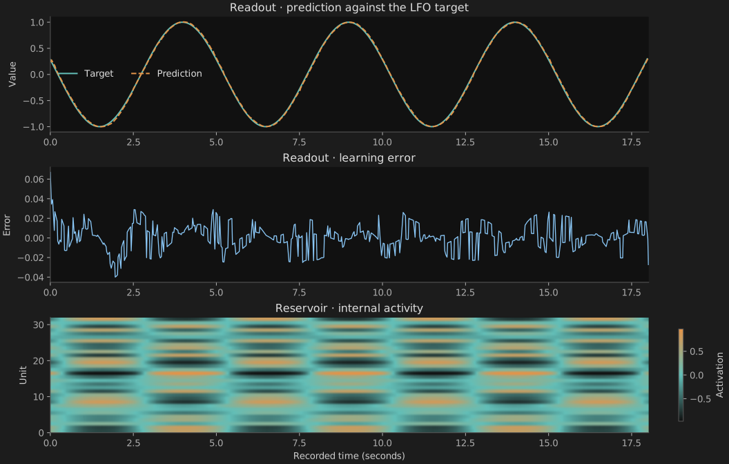
- LFO sends a single changing value to Reservoir.input and Readout.target.
- Reservoir.state feeds Readout.state. Watch prediction and error as learning runs.
- Turn readout/learning off to freeze the weights.
LFO.outReservoir.inputLFO.outReadout.targetReservoir.stateReadout.stateReservoir.stateReservoirGraphics.stateWhat to look for. The readout adjusts its weights to match the supplied target. It is learning from the current input, not forecasting a future one.
Freeze learning, then change LFO’s frequency. Compare error before and after enabling learning again.
Reset Readout after changing reservoir size or starting a new learning task. Keep target timing aligned with the state you want to train on.
Populations, spikes, and quantum states
Compare three independent models and the different kinds of data they produce.
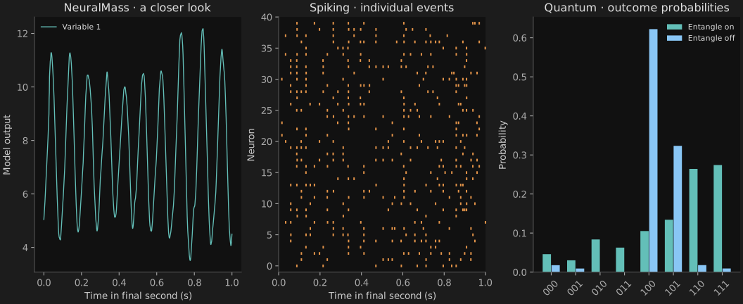
- Inspect NeuralMass.out as a line: its variables describe neural populations.
- Inspect Spiking.rate and the matching graphics output for individual spike activity.
- Inspect Quantum.probabilities and its graphics view while changing quantum/angle.
Spiking.spikesSpikingGraphics.spikesSpiking.potentialsSpikingGraphics.potentialsQuantum.blochQuantumGraphics.blochQuantum.probabilitiesQuantumGraphics.probabilitiesWhat to look for. Each output belongs to its model. A population variable, a spike rate, and a probability are different quantities.
Increase neuron/drive on Spiking. Then leave that model alone and switch quantum/entangle off to explore the quantum model separately.
These are simulations for exploration. The patch uses a small spiking network and three simulated qubits to keep the starting workload modest.
Working practice
Reset for a fair comparison
Choose a fixed seed where available and reset between runs. Change one parameter at a time, then allow the model to settle before comparing.
Separate a model from its picture
Use the signal outputs for measurements. Graphics nodes are views of those outputs; their colours and display settings do not change the underlying simulation.
Start small
Begin with the supplied network and particle counts. Increase size only after the patch runs comfortably. Keep time step and output rate fixed while comparing model behaviour.